From Tokens to Concepts: Building a Local SAE Interpretability Lab on an M1 Mac
I started this project with a simple question:
Can sparse autoencoders (SAEs) surface meaningful features from a small open-weight language model, locally, in a reproducible way?
Then it evolved into something more useful: an interpretability lab I can actually run, iterate, and explore.
If you missed the first post, start here:
- Part 1: https://curtiscovington.com/posts/sae-interpretability-on-a-small-transformer/
This post is the continuation: in Part 1, I proved the pipeline worked. In this one, I pushed sparsity harder, compared top-k regimes, and built an interactive explorer so insights are easier to discover.
Why this matters
A lot of interpretability work is either:
- too infra-heavy to reproduce quickly, or
- too qualitative to compare rigorously.
I wanted both:
- reproducible runs,
- measurable transfer,
- and a practical UI for feature exploration.
All local. No paid APIs. No cloud.
Setup
- Model:
EleutherAI/pythia-70m-deduped(6 transformer layers) - Activation target: one layer at a time, MLP output stream
- Data domains:
- A: wiki/prose-style text
- B: Python-heavy code corpus
- Token budget: ~100k tokens per domain per layer for collection (A and B each)
- Hardware: Apple Silicon (M1), MPS with CPU fallback
- SAE family: top-k sparse SAE (plus earlier ReLU+L1 baseline)
Experiment 1 recap: layer sweep
I trained SAEs across layers and evaluated:
- reconstruction (R² / MSE),
- sparsity (L0/L1),
- transfer degradation (A→B, B→A).
Protocol note: each SAE run uses a 90/10 split of collected activations per domain (train/val). Reported A_A and B_B are on held-out validation activations for the same domain; A_B and B_A are cross-domain evaluations using those trained SAEs.
Best layer in sparse sweep: Layer 2 (strong reconstruction + transfer balance).
That gave me the next question:
If sparsity is the point, where is the sweet spot for top-k?
Experiment 2: top-k sweep (k=48, 24, 16) with larger dictionary
I pushed dictionary width to 2048 features and swept:
- k = 48
- k = 24
- k = 16
Key result
The best overall configuration was:
k=16, layer=2
- A_A R²: 0.962
- B_B R²: 0.987
- A→B ratio: 1.69
- B→A ratio: 2.00
- L0: 16
- A_A MSE: 0.0183, A_B MSE: 0.0310
- B_B MSE: 0.0149, B_A MSE: 0.0299
(Transfer ratio definition: A→B ratio = MSE(train on A, eval on B) / MSE(train on A, eval on A) and analogously for B→A.)
In short:
- higher k preserved slightly more raw reconstruction,
- but k=16 gave better sparsity/transfer tradeoff and became the strongest overall score in this framework.
That’s a real win for this direction.
What kinds of features appeared?
When I inspected top features and contexts:
Code-leaning features
- import/module wiring patterns
- parser/token/AST metadata (
lineno, offsets, parse-version flows) - exception and guard-control flow (
except,raise, returns)
Prose-leaning features
- historical/biographical narrative fragments
- institutional/reporting language
- entity/topic clusters
Not perfectly monosemantic yet — but clearly more structured than random latent noise.
A quick caveat: on a small model at this scale, many features are still fuzzy and mixed compared to clean human-level concepts. That’s expected. The next frontier is scaling this lab to larger models (and better hardware) so concept structure becomes sharper and more semantically stable.
New pivot: from static plots to an explorer
Raw PCA plots (PC1, PC2) are useful, but not intuitive alone.
So I built an interactive feature explorer in the repo:
- map view (2D/3D feature map),
- selectivity filters (A-leaning / B-leaning / shared),
- feature inspector with top contexts by domain,
- nearest-feature navigation,
- cluster concept summaries.
This changed the workflow from: “look at one static chart” to “browse neighborhoods, inspect, and discover concepts.”
That’s the biggest practical shift: this is now a tooling foundation, not a one-off notebook result.
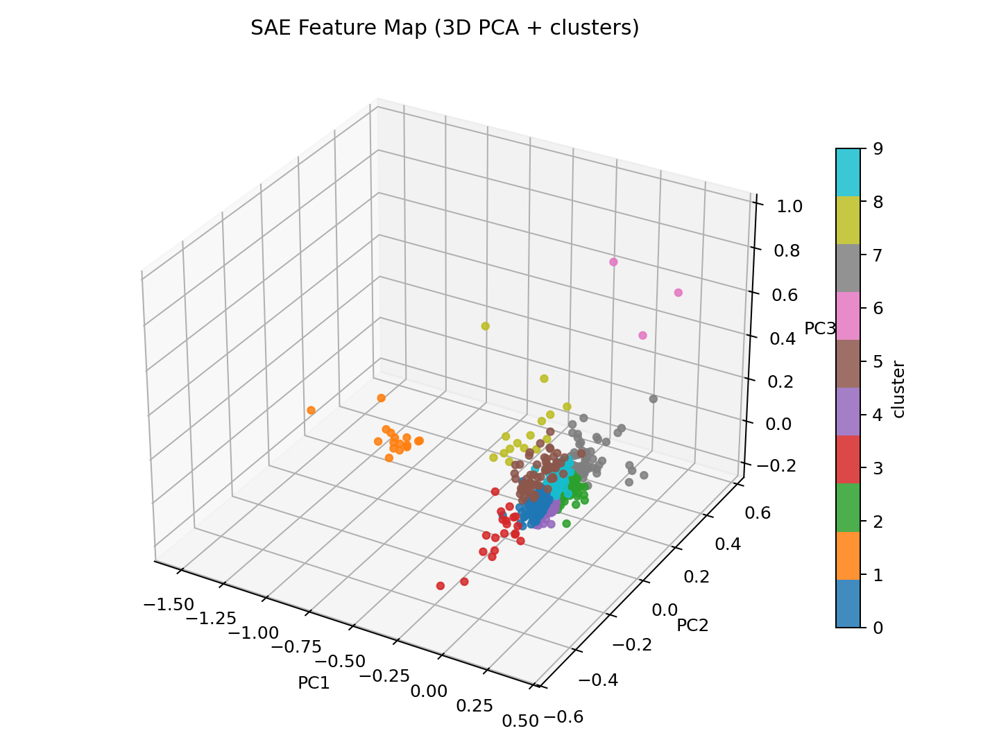
3D concept map (k=16, layer=2)
This is the feature-space concept map from the best run. Each point is an SAE feature; nearby points tend to behave similarly and often share concept-like patterns.
For this map, each feature vector is constructed from the SAE decoder row for that feature (its learned output direction in model space) concatenated with a small selectivity/statistics embedding (freqA-freqB, magA-magB, freqA, freqB). I then project those feature vectors to 3D with PCA.
Cluster colors come from k-means with k=10 on the PCA-reduced feature vectors using Euclidean distance. k=10 was chosen as a practical visual granularity for exploration (not heavily tuned).
What I learned
- Sparse-first objectives work — pushing top-k down exposed better tradeoff structure than stopping at dense recon quality.
- Layer matters — early/mid layers can dominate transfer/sparsity balance.
- Interpretability needs UX — if you can’t inspect neighborhoods and contexts quickly, you won’t extract insight.
Limitations
- Single small model (70M), single architecture family.
- Domain corpora are lightweight and intentionally constrained.
- Labels are heuristic, not human-annotated concept taxonomies.
- No causal intervention tests yet in this phase.
Next steps
- Add feature intervention experiments (suppress/amplify, measure output/logit shifts).
- Expand domain matrix (add a third corpus type).
- Improve concept labeling pipeline (semi-automatic + human curation).
- Track longitudinal runs in “lab mode” with saved findings cards.
TL;DR
This started as an SAE experiment and became a local interpretability lab.
And the current best result is clear enough to act on:
Top-k = 16 (layer 2, d_sae=2048) is the best current sweet spot for sparse, transferable features in this setup.