Interpretability via Sparse Autoencoders on a Small Open-Weight Transformer

I wanted to answer a practical question: can we get meaningful interpretability signal from Sparse Autoencoders (SAEs) on a tiny open model, locally, in a few hours?

Short answer: yes—with caveats.

I ran an end-to-end SAE probing pipeline on EleutherAI/pythia-70m-deduped, extracted a single layer’s activations, trained SAEs, and evaluated transfer between two contrasting corpora:

• A (general text): WikiText-2 training text (raw public text source)
• B (code): Python-heavy source text (CPython + Flask + NumPy files from public GitHub raw URLs)

The full run produced reproducible metrics, feature summaries, and figures suitable for this post.

Why this experiment matters

A lot of interpretability writeups either:

1. depend on large infra / custom kernels, or
2. stay qualitative with no measurable transfer story.

I wanted the opposite:

• Local-only (Apple Silicon MPS + CPU fallback)
• Re-runnable (pinned deps, fixed config, one command, fixed seed)
• Quant + qual together (MSE/R²/L0/L1 + concrete feature examples)
• Generalization test (train on A, evaluate on B, and vice versa)

That last one matters: if features only work in-domain, they’re less useful as interpretable building blocks.

Setup (condensed)

• Model: EleutherAI/pythia-70m-deduped
• Layer/stream: layer 3, MLP output
• SAE: linear encoder/decoder, ReLU hidden, MSE + L1 sparsity penalty
• Token budget: 120k tokens for A, 120k for B
• Hardware target: M1 MacBook (MPS), CPU fallback enabled

Note: MPS training can have minor run-to-run variation even with fixed seeds; expect close but not bit-identical metrics.

I ran two major passes:

1. Baseline SAE (weaker sparsity pressure)
2. Sparser SAE (stronger L1 + slightly smaller dictionary)

Core result (sparser run)

After increasing sparsity pressure (l1_coeff up, d_sae down), I got these metrics:

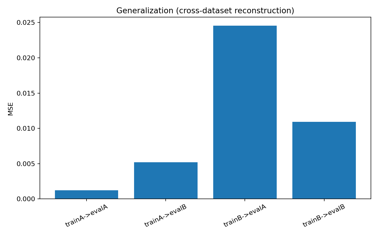
• Train A → Eval A: MSE 0.001241, R² 0.9911, Avg L0 619.65
• Train A → Eval B: MSE 0.005195, R² 0.9681, Avg L0 589.16
• Train B → Eval A: MSE 0.024533, R² 0.8244, Avg L0 563.66
• Train B → Eval B: MSE 0.010940, R² 0.9329, Avg L0 595.80

Generalization degradation ratios:

• A→B / A→A MSE: 4.19x
• B→A / B→B MSE: 2.24x

So transfer isn’t symmetric. The feature basis learned from A generalizes differently than the basis learned from B.

Visuals

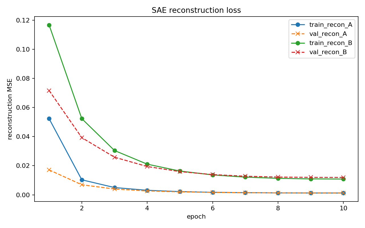
Reconstruction curves

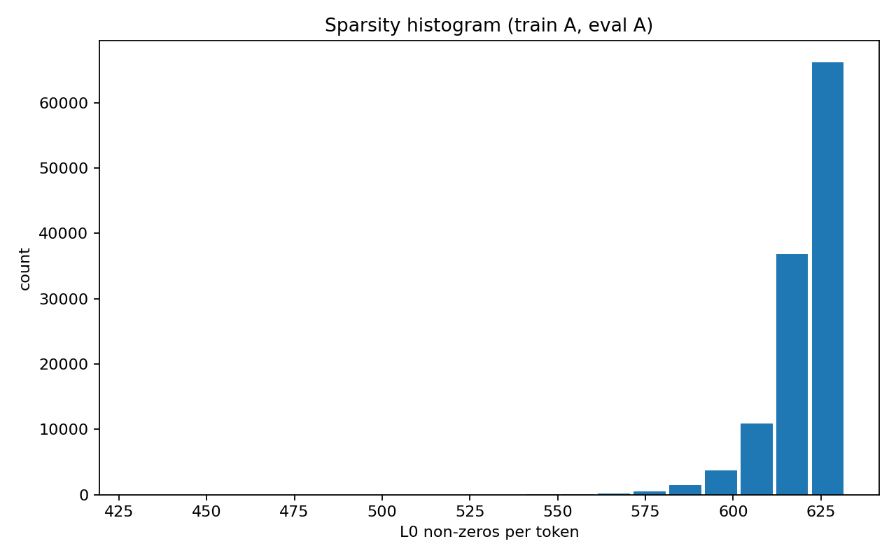
Sparsity histogram (L0 per token)

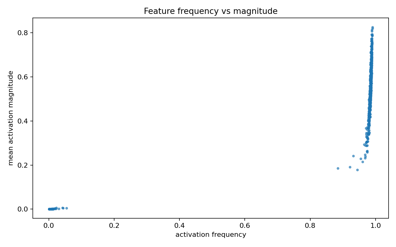
Feature frequency vs magnitude

Cross-domain generalization bars

What kinds of features appeared?

Code-trained SAE: clearer, more local patterns

Top features frequently aligned with recognizable programming motifs:

• import / from / werkzeug.exceptions
• none / raise / return
• error / return / filename
• import / elif / error

These looked like parser + control-flow + framework-error pathways.

Wiki-trained SAE: broader discourse/entity clusters

Top features were less surgical and more corpus-genre/entity flavored:

• miss / universe / 2006
• international / survey
• chronology/connective-heavy patterns (years, based, that)

Useful, but often less crisp than code features.

What improved after pushing sparsity?

Compared to the previous run, average L0 dropped significantly (from ~747–826 down to ~564–620 non-zeros/token), which is what I wanted. Reconstruction degraded slightly, but remained strong overall.

That tradeoff is expected:

• more sparsity → better feature selectivity
• but usually a reconstruction cost

Limitations

This is still an MVP interpretability experiment:

• single model, single layer, single stream
• no causal interventions yet (just probing/reconstruction)
• heuristic feature labels (no human annotation pipeline)

Next steps

If I continue this line, I’d prioritize:

1. Top-k SAE objective (instead of ReLU+L1 only)
2. Layer sweep (compare early/mid/late layers)
3. Feature intervention test (activate/suppress feature and inspect output shifts)
4. Cleaner corpus controls (reduce accidental topical leakage)

TL;DR

You can run a serious SAE interpretability workflow on a laptop, get strong reconstruction, and quantify transfer across domains. The most useful insight wasn’t just “it reconstructs”—it was how feature behavior shifts under domain transfer and stronger sparsity pressure.